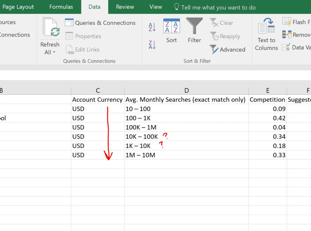
Have you ever downloaded an Excel sheet of keyword ideas from Google AdWords Keyword Planner? Since 2016, Google has change the Search Volume statistics (“Avg. Monthly Searches”) from single whole numbers (ie. “100”) to showing ranges instead (ie. “1K – 10K”).

Sorting Ranges Can Be Difficult
As you probably can guess, sorting with these columns may yield odd results. The below are ranges sorted in ascending order. Notice anything strange?
10 – 100
100 – 1K
100K – 1M
10K – 100K
1K – 10K
1M – 10M
The cell “10K – 100K” is now before than “1K – 10K” in ascending order. This is because Excel will sort this text in “Alphabetical Sort Order” instead of “Natural Sort Order“. In the former sort, numbers (ie. “0”) are placed before letters (ie. “K”). So since “10K – 100K” and “1K – 10K” have the same first character “1”, then we sort by the second character “0” and “K”.
How Do We Fix This?
First, we’ll need to use a new column to extract whole number values into. Double click the first cell in the new column to paste the following formula in. You’ll need to replace both cell references “D2” in the following formula with the cell you are trying to fix.
=SUBSTITUTE(SUBSTITUTE(LEFT(D2,FIND(" ",D2)),"K","000"),"M","000000")
Once you have that working, just copy and paste the cell down to the remaining rows. By default, it should use the relative row references as you copy and paste. You can also simply drag the bottom-right corner of the cell you want to copy down into the rows you want to paste into.
Once you have the new column working with the whole number values extracted, just sort your sheet with that column.
How Does This Formula Work?
This formula uses a combination of LEFT, SUBSTITUTE, and FIND functions.
What the SUBSTITUTE function does is it simply searches a text for a text you specify (old_text) and replaces the found text with a text you specify (new_text).
SUBSTITUTE( text, old_text, new_text )
The LEFT function takes only a portion of a text starting from the left and to the right as many characters as you specify (number_of_characters).
LEFT( text, number_of_characters )
The FIND function gives you the position of the first occurence of the text you specify (find_text) inside another text (within_text). If the start of the text you’re looking for is the first character, then the position is 0. If it starts from the second character, then position is 1, and so on. Another way to say this is that how many characters do we have to skip to find the text we are looking for (find_text).
FIND( find_text, within_text )
So Let’s Break Down The Formula
=SUBSTITUTE(SUBSTITUTE(LEFT(D2,FIND(" ",D2)),"K","000"),"M","000000")
Let’s add some spaces to help up see better.
= SUBSTITUTE( SUBSTITUTE( LEFT( D2 , FIND( " " , D2 ) ) , "K" , "000" ) , "M" , "000000" )
Let’s look at the most inner (“nested”) function.
FIND(" ",D2)
Let’s first replace the reference here with an example value for our demonstation purposes. Let say D2 references a cell with the range .
FIND(" ","10K – 100K")
The FIND function will look for the first space (” “) in the range value (“10K – 100K”) and return the position. The result of this function is 3.
3
Let’s step out a bit and see the function using this result and replace our FIND function with 3.
LEFT(D2,FIND(" ",D2))
becomes…
LEFT(D2,3)
Let’s again replace the reference with our example.
LEFT("10K – 100K",3)
Remember, the LEFT function takes a portion of the text. Conveniently, 3 is already the number of characters before the space that we only want (“10K”). Now we are left with just that.
"10K"
Let’s step out again and to see the next outer formula.
SUBSTITUTE(LEFT(D2,FIND(" ",D2)),"K","000")
Let’s replace it with what we know now.
SUBSTITUTE("10K","K","000")
The SUBSTITUTE function here will replace the “K” with “000” (thousand), giving us a whole number. Now we have this.
"10000"
One more step out and we are back at the beginning.
=SUBSTITUTE(SUBSTITUTE(LEFT(D2,FIND(" ",D2)),"K","000"),"M","000000")
Let’s replace with what we now from previous steps.
=SUBSTITUTE("10000","M","000000")
Here, this last SUBSTITUTE function will do nothing because there is no “M” (million) found to replace. So we are just now left with
="10000"
Sometimes we will be dealing with K (thousand) and sometimes M (million) so we will need to check for and replace both.
The Formula Once Again
=SUBSTITUTE(SUBSTITUTE(LEFT(D2,FIND(" ",D2)),"K","000"),"M","000000")
Remember to replace the two cell references (D2) in this formula above with the actual cell reference in your Excel sheet. Copy and paste this formula in a new column with relevant references to extract whole number values. After that, just sort the sheet with this new column.
I hope you find this helpful. If you have any questions or feedback, please feel free to comment below or contact us!
A Simpler Way
A simpler way is to replace your ranges of search volumes (“buckets”) with more accurate whole numbers instead.
Twinword Ideas is a keyword research tool that gets its data from Google, the same data that goes into Google AdWords Keyword Planner. On top of that, it shows whole numbers instead of ranges for average monthly searches. So what you can do is to use the import tab of Twinword Ideas and just copy and paste your keyword list from Keyword Planner and get whole number search volume statistics.
To use the import tab, simply click on the box that either says “Get keyword suggestions” or “Get statistics only” (marked red in the screenshot below), and change it to “Get statistics only”. Now you can paste your keyword list into the search bar and click on import.

On top of that, this tool provides AI-powered features to help you sort and filter your keyword list faster than going keyword by keyword. Check it out for yourself!


